So you’ve finally decided enough is enough. Dealing with landlords and apartments has become too much of a hassle, and its about time to start investing your money in something important. It’s time to buy a house.
 Looks like a nice place!
Now it’s time to start investigating some listings. If you choose to look online, you may find some super helpful websites like Zillow. One common feature is the predicted price, or as it’s known in Zillow, the “zestimate.”
Some of you may be wondering how exactly these companies come up with their estimates. It may seem obvious that they include things like the number of bedrooms, the number of bathrooms and the size of the house and property, but what else is included? How much influence does the kitchen have? What about a basement or a garage? Or the shape of and property and if there are any hills?
In this project, I sought to answer some of these questions by building a model to predict the price of a house. This project was based on a Kaggle competition.
Defining the Problem:
As this was a kaggle competition, the problem definition was provided for me as follows: “The website Zillow wants to create a “market value” tool that will allow customers using their site to see an estimated price for any home they list on the site. This tool should be able to generalize to all houses within the city of Ames, Iowa.”
Gathering Data:
Again, because this was a kaggle competition, data was provided in the form of two .csv files, a training data set and a testing data set. The csv file contained information on approximately 2,000 houses that were sold between 2005 and 2010 in Ames, with 80 features given for each sale. There was also a holdout set of approximately 900 houses provided to evaluate the strength of my model.
Exploratory Data Analysis:
Once we’ve obtained our data (thanks again kaggle!), the first thing to do is some quick investigation into what exactly we are dealing with. The table below shows some basic information for the training and testing data sets.
| Rows | Columns | Nulls | |
|---|---|---|---|
| Training | 2051 | 81 | 9822 |
| Testing | 879 | 80 | 4175 |
One of the first things I did was to check for null values, and there were a bunch of missing pieces of information. The graph below shows the percentage of missing data from the six categories with the most null values in both the training and testing set.
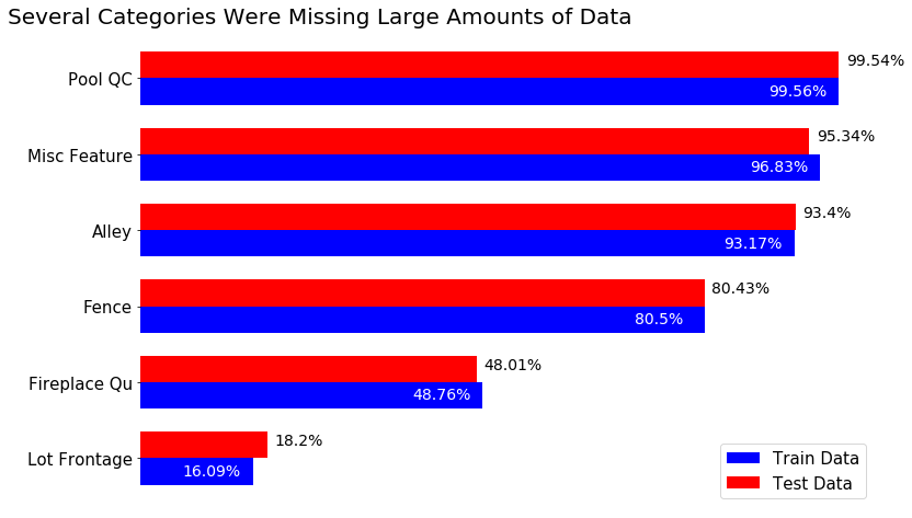 Percentage of values that were null by category in train and test set
Because of the extreme number of missing values in the Pool QC, Misc Feature, Alley, and Fence features, I decided to drop these from both the training and testing dataset. For Pool QC and Misc Feature, the information captured in these variables could also be seen in the Pool Area and Misc Feature Value variables respectively.
There were other categories that also contained missing values; in total 26 different categories were missing values. Thus began the process of cleaning the remaining 77 features within the data set.
Data Cleaning
 Cleaning is fun!
Before doing any modeling, all data must be numeric. Considering that this data set started with about half of the data entered as strings, data cleaning was a pretty hefty piece of work. There were several quality and condition rating columns that ranked specific parts of a house on a scale from poor to excellent. Since these are ordinal categorical values, I decided to convert the ratings to numerical values and treat them as continuous variables. Next I created dummy variables for as many of the categorical features as I could. After dropping a few specific observations with many null values, I was left with three variables with a large number of null values: Mas Vnr Area, Gar Yr Blt and Lot Frontage.
The null values in the masonry veneer area category represented houses that did not have any masonry veneer, so it was an easy decision to replace the missing values with zeros. The garage year built and lot frontage variables were considerably more complicated.
First I looked at the garage year built and saw that null values represented houses without garages. Then I looked at the houses with garages for the distribution of years garages were built, and the relationship between garage year and sale price.
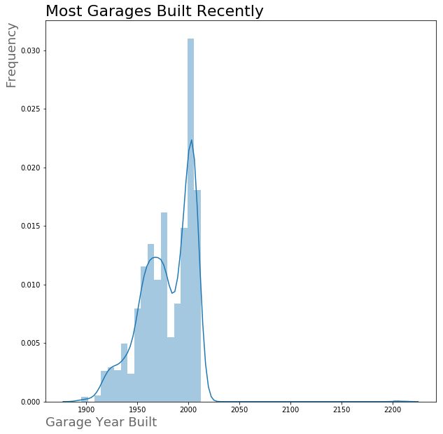 The distribution of Garage Year Built is severely left skewed
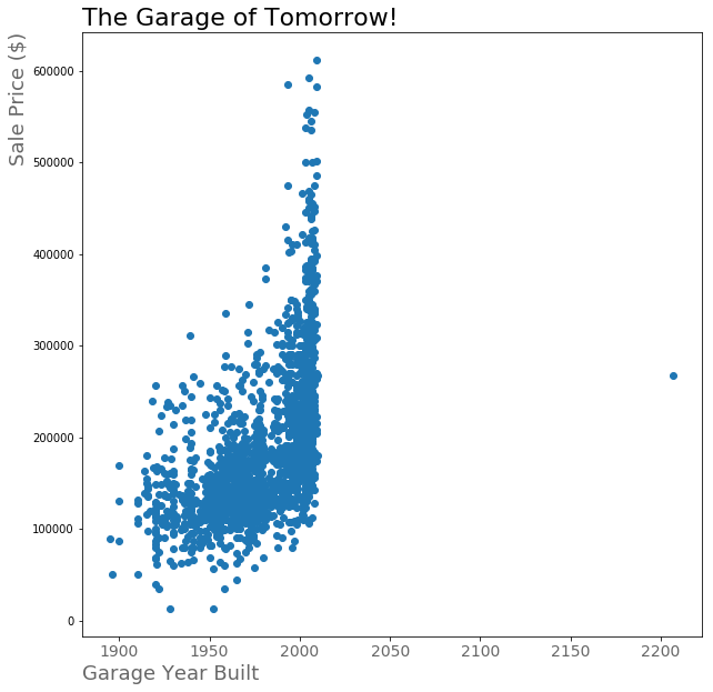 There seems to be a positive correlation between Garage Year Built and sale price…hey what about that garage from the future?
So first things first, we can’t have a house with a garage built 200 years from now (unless Doc and Marty have started a time traveling construction business). Since the house was remodeled in 2007 and the garage year built was 2207, I assumed this was a data entry error and replaced 2207 with 2007.
For the remainder of the houses without garages, the question of what year to use for this category was a tough one. Using the year that the house was last remodeled or the year the house was built would artificially inflate the price of newer houses without a garage and artifically deflate the price of houses with older garages. Using a 0 would not make sense, as it would drastically lower the correlation between the year a garage was built and the sale price of a house. Instead, I decided to use 1918.5, which is the minimum value for garage year built that was not an outlier.
Last up was the lot frontage. Since I did not want to just use the average value of the lot frontage, I decided to try and predict the values of the lot frontage using linear regression. I used all variables except for Lot Frontage, SalePrice, PID, and Id as predictor variables. I made the set where the Lot Frontage was null into my holdout set and did a train/test split on the remaining data. I then tested out a multiple linear regression, a lasso regression, and a ridge regression by fitting to the training data and scoring on the testing data. The ridge regression had the best performance, so I used predictions from the ridge regression to fill in the missing values for both the training and testing sets.
Feature Selection
Now that all of the data is clean, we can finally jump into selecting features. For my first model I wanted to keep things simple, and decided to start with just a few feature that had the strongest correlation with sale price. First, I had to determine which features had the strongest correlation with the sales price.
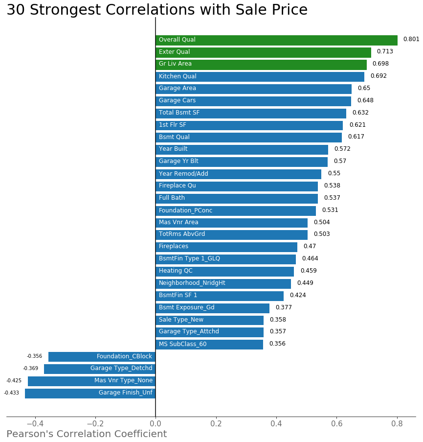 Is anyone surprised by these features?
For my first model, I decided to include the three categories with the strongest correlation with sale price, which are highlighted in green on the graph above.
Modeling
Now it’s finally time to model!
 Fierce!
Model 1
Multiple Linear Regression Using 3 Variables
The first model was a mulitple linear regression with just those 3 variables from the graph above. Before modeling, we have to train/test split our data so that we can evaluate the effectiveness of the model against unseen data. For this model, I created a train/test split with a ratio of 80/20, so that the model was fit against 80% of the data and then evaluated against the remaining 20% it had not yet seen. After fitting the first model, I created the scatterplot below of predicted vs. actual price.
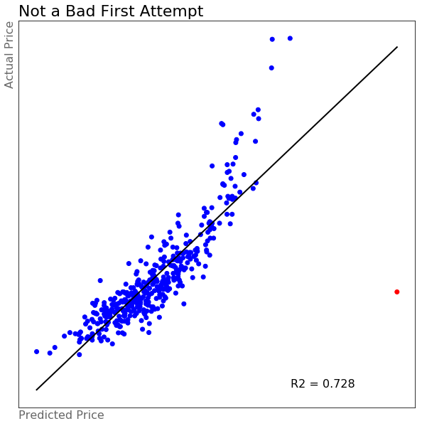 Who would have thought such a simple model would do this well?
The first model had an R2 score of about 0.728, meaning the model explained just under 73% of the variance in the data. Not a bad start at all. Except, what exactly is happening with that point outlined in red? That is predicted to be waaaay too expensive. Clearly we need to consider more than just these three variables.
Model 2
Model 1 + Neighborhood dummy columns
My next thought was that the neighborhood that a house is in must have a significant effect on the value of the house. This can give insight into how good the schools are, what amenities the house is near, and many other insights. For this second model I used the same three variables from the first model and added in all of the neighborhood dummy variables.
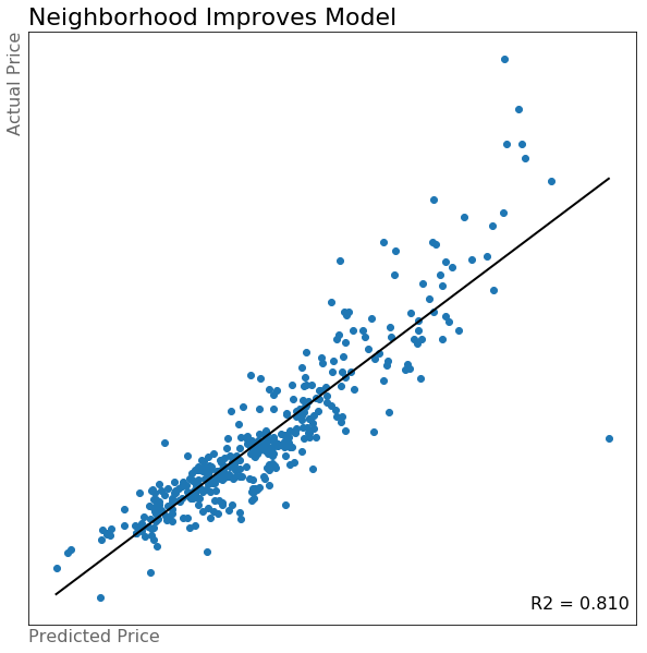 Neighborhoods really improve the model! Think about all the information that neighborhoods capture
The R2 score increased to approximately 0.810, an increase of about 8%. We can still get to be even more accurate though.
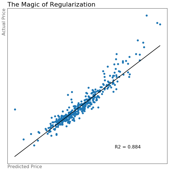
Model 3
All features With Lasso Regularization
At this point, my impatience has started to kick in. I know that I can slowly go through all of my features and meaningfully choose those that will increase the fit of my model, but that sounds like it will take a really long time and a lot of effort. This is where I start looking for shortcuts. Model 3 used all 256 of the features that I created. In order to make sure that the noise within the data does not outweigh the signal, this is when I start to harness the power of regularization.
Regularization adds a penalty to the loss function that is used to determine the best coefficients for the regression model. This helps to prevent overfitting of the model on the training data that would prevent the model from being able to generalize to unseen data. In this model I used Lasso regression, also known as the l1 penalty because it the more “brutal” of lasso and ridge. This model was the best yet, as seen in the scatter plot below.
 It just keeps getting better!
Even with this model, I still felt there was room for improvement. After all, when you go to look at a house you don’t consider each piece in isolation, but rather take a more wholistic view on the house. In order to capture this in the data, I decided to investigate some interaction terms. An interaction term is created by multiplying the values of two different variables.
Model 4
Interaction Terms Through PolynomialFeatures.
There are multiple ways to make interaction columns, but one really convenient way is using the PolynomialFeatures module from the sklearn package. This module allows you to create all possible interaction features from a given dataframe for any degree you choose. I decided to limit this to only the second degree, as it gave me about 60,000 features to work with. With so many features, regularization was a must. Again I chose to use lasso regression and ended up with the following model.
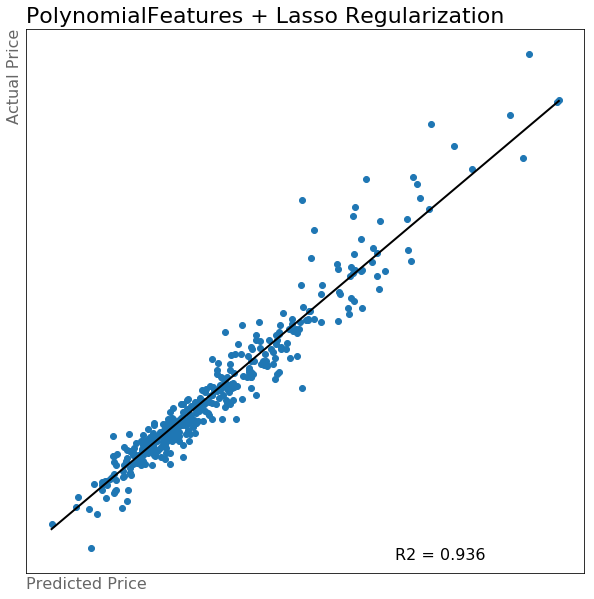 This one was worth the wait…all 45 minutes of it
As I was running this model, I realized a couple of things. One important one is that this model took a really long time to run. Because of all of the features, it was very computationally and time intensive. While it may have been a very accurate model, it did not seem like the best use of resources in predicting housing prices. I knew that after regularzation there would be only about 1,000 features remaining to deal with. Instead of just using this model, I decided to look for better ways to create some of these more meaningful interaction terms.
Model 5
Interaction Terms Through Custom Functions
Instead of using all of the second degree interaction terms, I wanted to have the opportunity to more meaningfully select interaction terms. To do so I wrote three separate custom functions.
best_interaction_finder: This function took in a string and generated a list of all the columns that contained that string. It then looked for which interaction feature, out of all possible interaction features, had the strongest correlation with sale price. For example, calling the function with the string ‘Garage’, would first create a list of all of the features that contained ‘Garage’. Then it would generate all possible interaction terms between those features and determine which one was most strongly correlated with sale price. It would then add this interaction feature to the train/test split data from the original training set as well as the holdout data. An example of the interaction feature generated with the string ‘Garage’ is shown below.
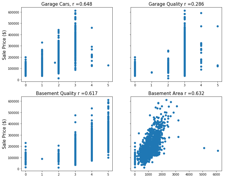 All four original features seem to have a moderate positive correlation with sale price
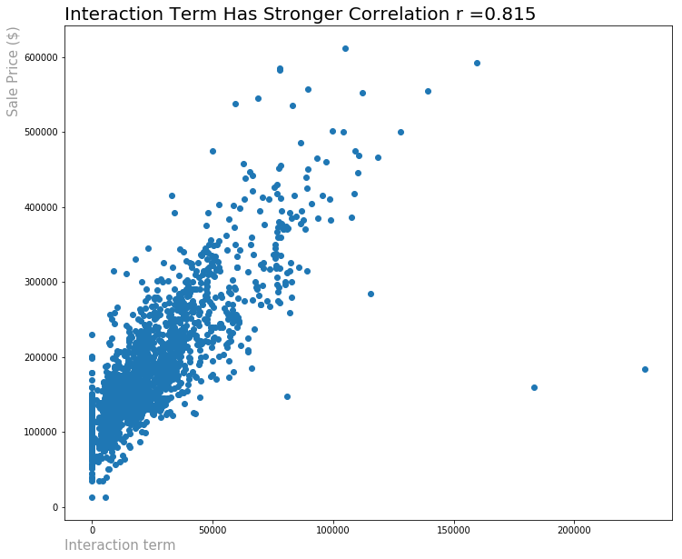 The interaction term between all four has the strongest correlation with sale price
-
best_degree_2_interactions: This function takes in a number, n, and determines the list of n strongest interaction features by correlation with sale price. For example, calling this function with an input of 500 would determine the 500 strongest 2nd degree interaction features by the interaction features’ correlation with sale price. It would then append these 500 interaction features to all the necessary data frames. -
strong_2d_interactions: This function takes in a float value between 0 and 1 and determines all interaction features with a correlation coefficient that had an absolute value greater than that parameter value. So if you called this funciton with the value 0.6, the function would determine all interaction terms with a correlation coefficient above 0.6 or below -0.6 and add them to the necessary data frames.
After writing these custom functions, I tried using them by iterating through and testing out a variety of parameters. What I found was that the models I created were almost as accurate as my fourth models. As seen below, I created models with an R2 score of .
 Almost as good as the last model, in less than a third of the time!
Not only was this model nearly as accurate as my previous one, but is also took significantly less time to run and was much more efficient in terms of time and computational resources. I would need to know more information to determine whether the additional accuracy provided by model four was worth the extra resources it took to create model 4, but that decision would require the input of stakeholders.
Interpreting Results
When making my final evaluation of my models, I used the kaggle competition scoring to determine which model best represented the data. What I found was that my fourth and fifth models were very close in performance, scoring within 1000 points of each other as determined by the root mean squared error from the holdout set provided by kaggle. Despite their similarity in performance, the models ended up being quite different. The graphs below show the largest coefficients from each model.
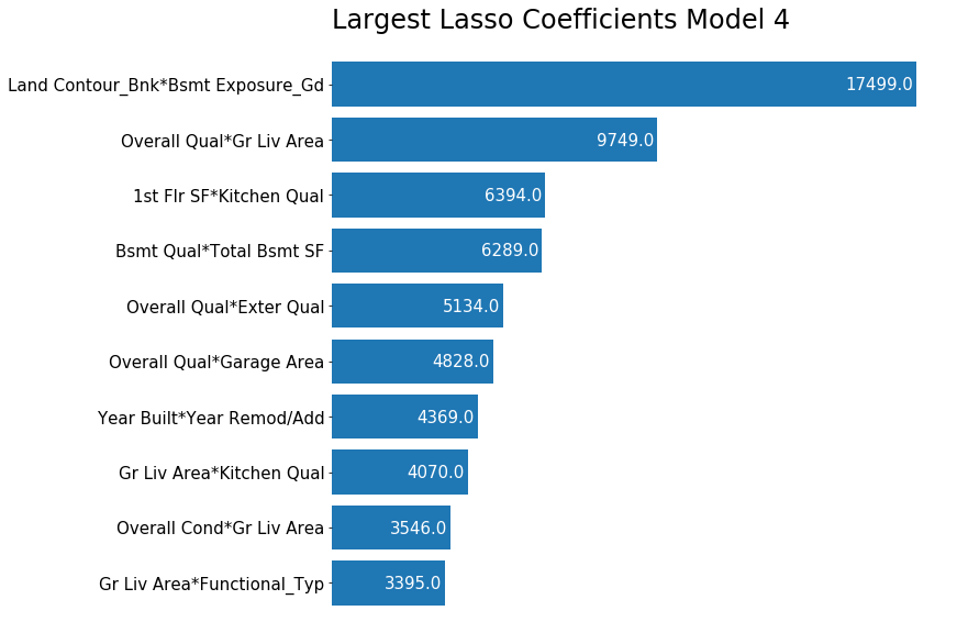 Largest Lasso Coefficients Model 4
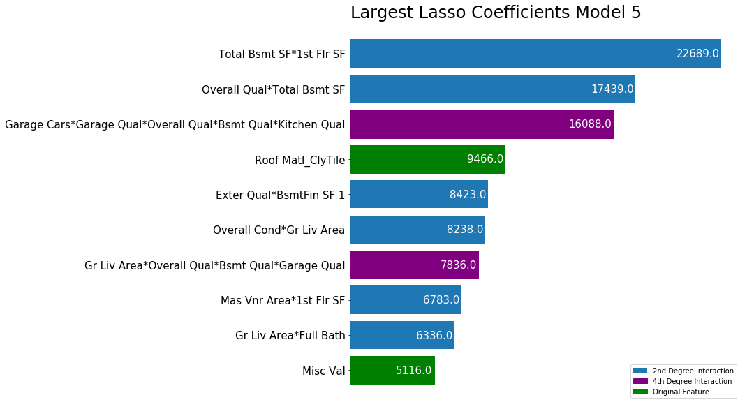 Largest Lasso Coefficients Model 5
The fourth model, which was based on all of the second degree interaction terms, primarily based its prediction on second degree interaction terms, with the top ten most important coefficients all being interaction terms. The fifth model had a diversity of term degrees for the ten largest coefficients; there were two original features, two fourth degree interaction terms, and six second degree interaction terms.
Next Steps
I would love to continue working with this data and this project to see if I can gain any more insights into housing prices in Ames. Some possible next steps are:
- Are there specific hyperparameters that we can identify and change in order to fine tune our model?
- This may be further tuning the lasso regression based on the PolynomialFeatures transformation, or determining which interaction features to use for model 5
- Does this model generalize to other cities? If so, which ones?
- There may be some things that are specific to Ames that are captured in the models created here, but without testing this model out on other cities it is impossible to know. Obviously, this would require revamping or dropping the neighborhood variables, but I would be interested to see which features generalized well and which did not.
- Can we categorize our houses in a specific way in order to build more accurate prediction models?
- This project involved looking at a large variety of houses. I would be curious to see if it was more effective to instead categorize houses into different groups and then build regression models for each group to see if it outperformed the more wholistic model.